Theorem Index
This page lists all mathematical theorems, lemmas, and corollaries found across the site. Click on any item to jump to its location in the notes.
The function
defined on is an inner product, and so ( a positive integer) forms an @inner-product-space.
Since is a field, is obviously a vector space.
To see that this is indeed an inner product, we'll show the required properties hold.
For @conjugate-symmetry, let and let Then,
and
and since is arbitrary, it holds for any respective pair of components in and and so
For @linearity in the first argument, let Then
Now, to show @positive-definiteness let Then,
(a) Suppose and
Then, converges to if and only if
(b) Suppose are sequences in is a sequence of real numbers, and Then
For (a), assume Then, from the definition of the norm,
that is, the distance from to is always less than or equal to the distance from to Therefore, for and we can pick to make this true for as small of as we'd like. Therefore,
Conversely, assume Let For some integer when we have
Therefore, implies that
so
Part (b) follows from part (a) and A sequence in converges iff its components converge.
Referenced by (2 direct)
The probability of or is the probability of plus the probability of minus the probability of and occurring together:
If and are mutually exclusive events,
We have to subtract the overlap between and to avoid double counting.
Similarly
The probability of and is the probability of times the probability of given , or equivalently, the probability of times the probability of given .
If and are independent, this reduces to .
When and are continuous and is smooth, we can calculate the value of the line integral by expressing and in terms of any parametric representation of and evaluating the resulting definite integral:
All parameterizations of the curve lead to the same value.
Assume a complex function is defined on a neighborhood of and is complex differentiable at Let and write Then all of the partial derivatives exist and
and
By assumption and definition of the complex derivative, we have that
Now, this limit must exist and be the same no matter what path we take. So, we can take the path along the real axis by setting and sending and we get
and hence,
This gives us that the partial derivatives and exist and
that is,
Now, we can repeat this trick by sending to zero along the imaginary axis by setting and sending to get
and hence
This gives us that the partial derivatives and exist and
that is,
Now, comparing (a) and (b) we have
If a smooth curve , is traversed exactly once as increases from to , the curve's length is
The arc length of curve in can be defined the same way, assuming :
Let be the set of all sequences whose elements are the digits and . This set is uncountable.
Let be a countable subset of and call the elements of We will construct a new sequence in the following way:
That is, the th digit of will be the opposite of whatever the th digit of is. So, differs from in the first digit, from in the second digit, in the third digit, and so on, so that it differs from all elements of and therefore is not contained in But, is definitely in since it its elements are the digits and Therefore, is a proper subset of so any countable subset of must be a proper subset of But, can't be a proper subset of itself, and therefore must be uncountable.
This approach to proving this theorem is due to Cantor and is called diagonalization, and the animation below illustrates why.
The set of real numbers is uncountable.
I won't give a full proof here, but this can be accomplished by considering the binary representation of real numbers in the interval consists of infinite sequences of and .
For complex and complex we have
If the series converges absolutely for any any complex including negative integers.
Other convergence conditions are listed here.
Referenced by (1 direct)
Direct references:
The expansion of any nonnegative integer power of the @binomial is a sum of the form
Every bounded sequence in contains a convergent subsequence.
Note that any bounded sequence is a subset of some closed set, bounded and thus compact k-cell in Therefore, is a sequence in a compact metric space, and has a convergent subsequence.
Every closed set in a separable metric space is the union of a (possibly empty) perfect set and a set which is at most countable.
Let be a separable metric space and be closed. If is at most countable, then we are done.
Suppose that is uncountable. Note that the proof of Suppose with uncountable,... only uses the property that is a separable metric space, and it therefore generalizes to any separable metric space. Thus is the union of a perfect set - its condensation points, , and a set that is at most countable,
Every countable closed set set in has isolated points.
Let be a countable closed set in Suppose for contradiction that has no isolated points. Then every point of is a limit point of and thus is perfect set. But, every nonempty perfect set in is uncountable, a contradiction. Thus, our assumption that has no isolated points is incorrect, and must contain isolated points.
The Cantor set contains no segment.
Suppose, for the sake of contradiction, that some segment and let Pick some such that Now, is the union of intervals of length and since it must be the case that is a subset of some interval of length However, this can't be the case, since by construction. Therefore, our provision assumption is incorrect, and contains no segment.
The Cantor set is compact.
Clearly, is bounded, for it lies within Each is composed of the union of closed intervals, and the union of finitely many closed intervals is also closed. is then the intersection of infinitely many closed intervals, which is again closed. Therefore, is closed and bounded, and by Heine-Borel, is compact.
The Cantor set is not empty.
Suppose has as an interval and thus Then, by definition, will contain and as intervals, so Note that has as an interval. By induction, all contain and , and therefore so does their intersection and is nonempty.
Referenced by (2 direct)
Direct references:
The Cantor set is a perfect set.
Let Let and pick to be large enough that Then, lies in one of the intervals of length in call it The endpoints of are also in (see The Cantor set is not empty.,) and at least one of them is not Since the endpoints are contained in a neighborhood of with radius all neighborhoods of are limit points of and therefore is perfect.
Because nonempty perfect sets in are uncountable, and the Cantor set is nonempty and perfect, the Cantor set is uncountable.
Referenced by (1 direct)
Direct references:
A sequence converges in if and only if it is a cauchy sequence.
Suppose converges. Then, because is a metric space, is cauchy.
If the derivative of a complex function is continuous in a domain containing a simple, closed, piecewise smooth curve and its interior, then
If is analytic in a @simply-connected domain then for every simple closed @path in
Let By the definition of the contour integral, we have
Because is analytic, the Cauchy-Riemann Equations tell us that and have continuous first partial derivatives, and therefore, we can apply Green's Theorem. Now, we can take the first integral and transform it
But, by Cauchy-Riemann Equations, so this integral evaluates to
Now, for the second integral, using Green's Theorem again, we get
and by Cauchy-Riemann Equations, so this integral also evaluates to which makes the overall integral as well.
A function is analytic in an open set if and only if the first partial derivatives of and are continuous on and satisfy the Cauchy-Riemann equations therein
In polar form, we have and set
so the condition is then
Referenced by (1 direct)
Direct references:
If is a real constant and are independent random variables with mean and standard deviation then
TODO: the precise statement is cut off in the source; complete it.
Referenced by (1 direct)
Direct references:
Let be drawn according to Then
From Chain rule for joint entropy, we have
Referenced by (1 direct)
Direct references:
The entropy (joint entropy) of the joint event is the entropy of plus the entropy of when is known, that is,
Note that
The first term on the RHS is just The second is
Altogether, we have that or
Referenced by (1 direct)
Direct references:
Referenced by (3 direct)
From Mutual Information and Entropy we have
Then, from Chain Rule for Entropy and Chain Rule for Conditional Joint Entropy we have, simplifying,
Now, from our definition of conditional mutual information we get
We use the Logarithm Change of Base here.
TODO: Cover & Thomas, Section 2.9.
Suppose and is a random variable with the finite mean and standard deviation Then
Intuitively, this means that the probability that is far away from its mean can't be too big.
Note that the upper-bound on this probability is proportional to the variance of the random variable and inversely proportional to the distance of from its mean. So, as the variance increases, the probability of taking on values further from its mean also increases, and as the distance from the mean increases, the probability of taking on values at least that far from decreases.
Also note that while Markov's Inequality only requires knowledge of the mean (the first moment), Chebyshev's Inequality requires knowledge of the variance (second moment). Also, Chebyshev's inequality works for any random variable with a variance defined, rather than just on non-negative random variables.
Let be a random variable with mean and variance . Define the non-negative random variable
By Markov's Inequality, for any , we have
Set . Then,
Since the variance of is , it follows that
Note that
Thus,
Referenced by (2 direct)
Direct references:
Closed orbits are impossible in gradient systems.
If we're always moving "downhill" in some direction in a space, it's impossible to come back to where we started. This is another reason why oscillations aren't possible in one dimensional systems.
If a line integral is independent of path in a domain , and is a closed, piecewise smooth curve in that contains only points of in its interior, its value is zero:
Closed subsets of compact sets are compact.
Suppose with closed relative to and compact. Let be an open cover of Since is open relative to (see A set is open iff its...), if we add it to we obtain an open cover of let's call it Since is compact, we can obtain a finite subcover of by discarding all but a finite number of sets from let's call it Since is also a finite subcover of and therefore is compact.
If we may, but aren't required, to exclude it, and still have a finite open cover of
If is closed and is compact, then is compact.
Because compact sets are closed and the intersection of two closed sets is again closed, is closed. Since and closed subsets of compact sets are compact, is compact.
Referenced by (3 direct, 1 transitive)
Direct references:
Transitive (depth 1):
Closure distributes over finite unions.
If then
Let Then, for some If then so If is in some then every neighborhood of contains some point and since so
Conversely, let If for some and thus If is only in suppose for contradiction that For each let be a neighborhood centered at with Then, is a neighborhood of (see (a) - For any collection of...,) but for all so But, this contradicts our hypothesis that so our contradictory assumption must be invalid, and
Any compact subset of a metric space is closed.
Suppose is compact relative to metric space Let For each we can define and let and be neighborhoods of radius around and respectively. Note that and are disjoint, because we defined their radii to be half the distance between them, and they are open.) Now, since is compact, we can pick a finite number of points in such that ( is a finite subcover of ) Using the same set of points as reference, let Note that since each is disjoint with its paired (to be in , a point must be in all but any point in is not in at least one ) is open, since it is the intersection of finitely many open sets (see (a) - For any collection of...) and obviously contains since each contains . Therefore, has a neigborhood that is disjoint with (since ), and is therefore an interior point of It follows that is open, and that is closed.
Referenced by (2 direct)
Every compact metric space has a countable base and is therefore separable.
Let be a compact metric space. Fix (any natural number will do,) then, consider the open cover of balls of radius centered at Now, because is compact, some finite covers
Now, consider the set of all balls for all
Because the union of a sequence of countable sets is countable, is countable. To show is a base for let be an open subset of and let Let such that Pick natural such that Then, for some (because no point in is more than away from the center of some and therefore is a countable base of Since we can make as close to as we like, the centers of are dense as well as countable, and are therefore a countable dense subset of so is separable.
Compact metric spaces are complete.
That is, if is a compact metric space and if is a cauchy sequence in then converges to some point of
Let be a cauchy sequence in the compact metric space For let bet the set consisting of Then
by two theorems above. Each is a closed subset of the compact space and is thus compact. Also, which implies that . Now, we have that there is a unique which lies in every
Let Since there is an integer such that if Since we have that for every and thus for every That is, if so converges to
Referenced by (1 direct)
Direct references:
Referenced by (2 direct)
Direct references:
Suppose Then is compact relative to iff is compact relative to
Suppose is compact relative to and that is an open cover of relative to such that We need to show that a finite subset of covers Because is open relative to and (see Suppose A subset ...) there are sets open relative to such that for each Now, since is compact relative to we have for some finite set of indices Now, since which shows is compact relative to
Conversely, suppose is compact relative to and let be a cover of open relative to We need to show there is a finite subset of that covers Let for each Then (b) will hold for some set of indicies, and since each (a) is implied by (b) and we've shown is compact relative to
The complement of an intersection is equal to the union of complements.
Let and be sets. We want to show that
Suppose Then, is not in that is, is either not in or it is not in or it is in neither. If is not in then it is in and therefore it is in The same approach works with and therefore and we have shown
The complement of a union is equal to the intersection of complements.
Let and be sets. We want to show that
Suppose Then, if or then and a contradiction. Therefore, and That is, and therefore
Referenced by (2 direct)
Let be a collection of sets. Then
Suppose Then, so is not in any Therefore, for every and thus Conversely, suppose Then, is in every that is, is not in any Therefore,
This is just De Morgan's law extended to arbitrary indexed collections.
Suppose are metric spaces, with
If is continuous at a point and if is continuous at the point then is continuous at
Let Since is continuous at there exists such that
Since is continuous at there exists such that
It follows that
if and Thus, is continuous at
Basically, since is continuous, we can control how close its output is to by controlling how close its input is to which we can certainly do, since is also continuous, and we can control how close its output is to by controlling how close its input is to
TODO: Cover & Thomas Theorem 2.7.4.
is a concave function of
Let be the uniform distribution on outcomes. Then from the definition of @relative-entropy,
Then, from the definition of cross-entropy
So,
and by Convexity of Relative Entropy, entropy is a concave function.
The intuition is that mixing distributions can never decrease uncertaintity.
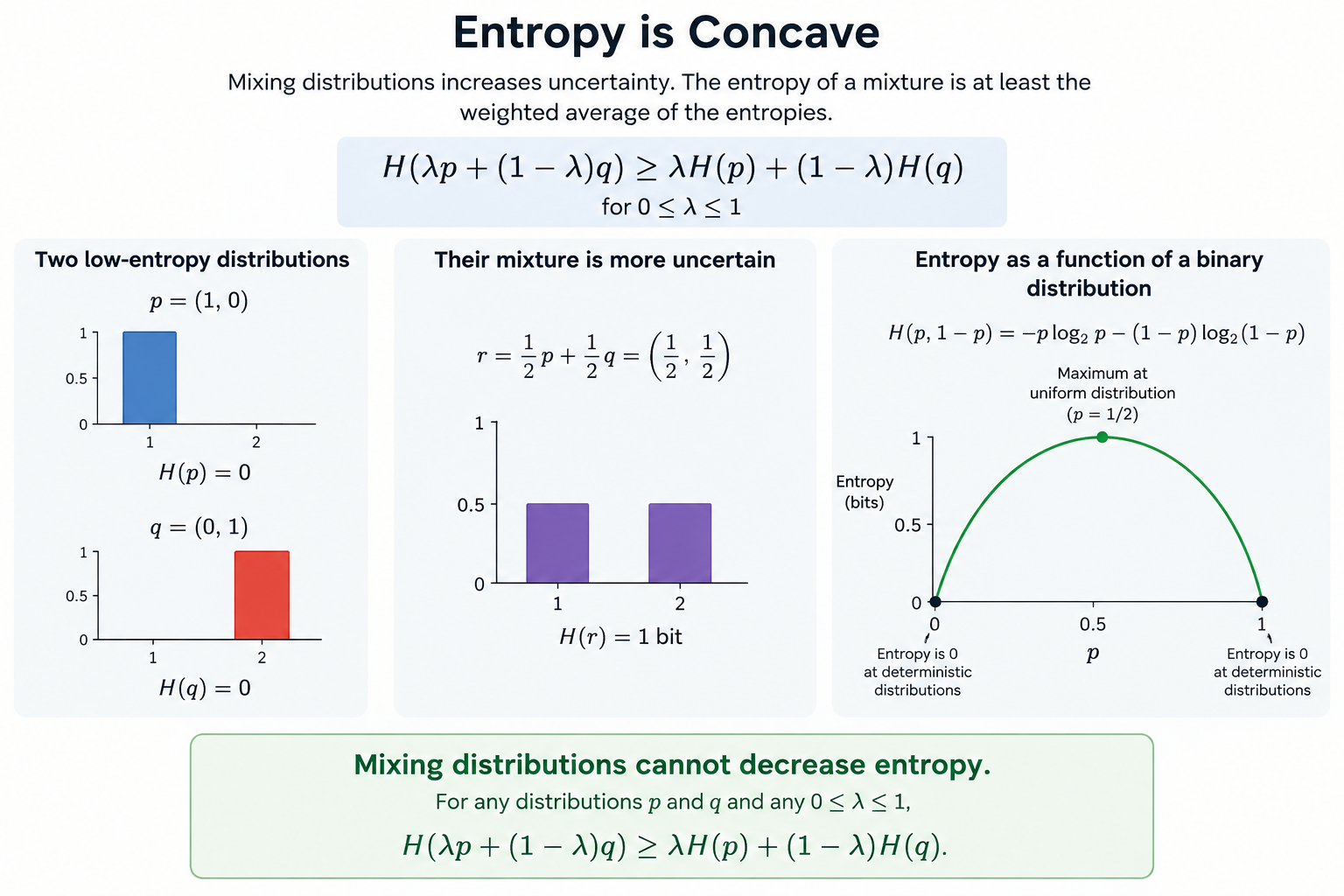 The image above was generated using GPT-5.6 Sol.
We already proved Uniform distribution maximizes entropy using Lagrangian multipliers, but the proof above shows it in another way. If then and since is constant in is maximized by .
Suppose with uncountable, and let be the set of all condensation points of Prove that is perfect and that at most countably many points of are not in that is, that is at most countable.
Let be a countable base of (see is separable. and Every separable metric space has a countable...,) and let be the union of those for which is at most countable. We will show that
Suppose Then is in no for which is at most countable, that is, every neighborhood of has uncountably many points in and thus
Conversely, suppose Suppose, for the sake of contradiction, that Then for some where is at most countable. But, since is an interior point of this there is a neighborhood and since every neighborhood of has uncountably many points in we have a contradiction, and thus our assumption that must be incorrect, and therefore and Furthermore, since is a union of open sets, is open, and is closed.
Since is open, only countably many are required to cover it. Each of these has at most countably many points in so has at most countably many points in that is, there are at most countably many points of that are not in
Now, to show all points in are limit points of suppose Let be a neighborhood of Then, is uncountable. Now, since there are at must countably many points in that are not in there are at most countably many points in and therefore there must be uncountably many points in Therefore, every neighborhood of contains infinitely many points in other than is a limit point of and is perfect.
Referenced by (1 direct)
Direct references:
If is the mean of a random sample of size from a population with a known variance , a confidence interval for is given by
If is the mean of a random sample of size from a population with an unknown variance, and the standard deviation of the sample is , a confidence interval for is given by
A subset of the real line is connected if and only if it has the following property: If and then
We will proceed both sides of the implication by proving the contrapositive, i.e., that if the interval property doesn't hold, then the set isn't connected, and conversely, that if the set isn't connected, the interval property doesn't hold.
Suppose and Then where
Since and they are nonempty, and since and they are separated. Therefore, is not connected.
Conversely, suppose, for the sake of contradiction, that is not connected. Then there are nonempty separated sets an such that Let and assume Define
By Let be a nonempty set of..., and because and are separated, Therefore
If it follows that and
If then hence there exists such that and (because means there is a neighborhood of that contains no points of .) Thus, and
If is used as an estimate of we can be at least confident that the error will not exceed a specified amount when the sample size is
TODO: the sample-size formula is missing from the source; complete this statement.
Conservative systems have no attracting fixed points.
Suppose were an attracting fixed point in a conservative system. Then, note that all trajectories in the basin of attraction approach as Since is continuous, the energy in the limit as trajectories approach is equal to the energy at the fixed point, and so the energy along the entirety of each trajectory is equal to the energy at the fixed point. But, this implies that the energy in the entire basin of attraction is the same as the energy at the fixed point, which violates our definition of a conservative system (i.e. we require that be nonconstant.) Therefore no such fixed point can exist.
Let be a sequence of random variables with moment generating functions defined by
for all for some .
Suppose there exists a function , finite for , such that
for all , and that is the moment generating function of some random variable .
Then the distributions of converge in distribution to , i.e.,
If converges, then is bounded (sequence).
Let Only finitely many points in lie outside of . That is, for some integer only the points where lie outside of Let Then, for all
TODO: Cover & Thomas Theorem 2.7.2.
is convex in the pair that is, if and are two pairs of probability mass functions, then
for all
First, note that the set of probability mass functions on is the set of probability vectors in where and thus is a convex set. takes a pair which is again convex, so is defined on a convex set.
Now we'll apply Log Sum Inequality to the one term with a fixed left-hand side of the inequality in the theorem, but we'll do some replacements to make it more obvious what's happening.
Let
Using those substitutions, with Log Sum Inequality, we have
Summing both sides of this over gives us
relative-entropy is a convex @surface over @pairs , with a flat-bottomed zero valley along , rising as and differ.
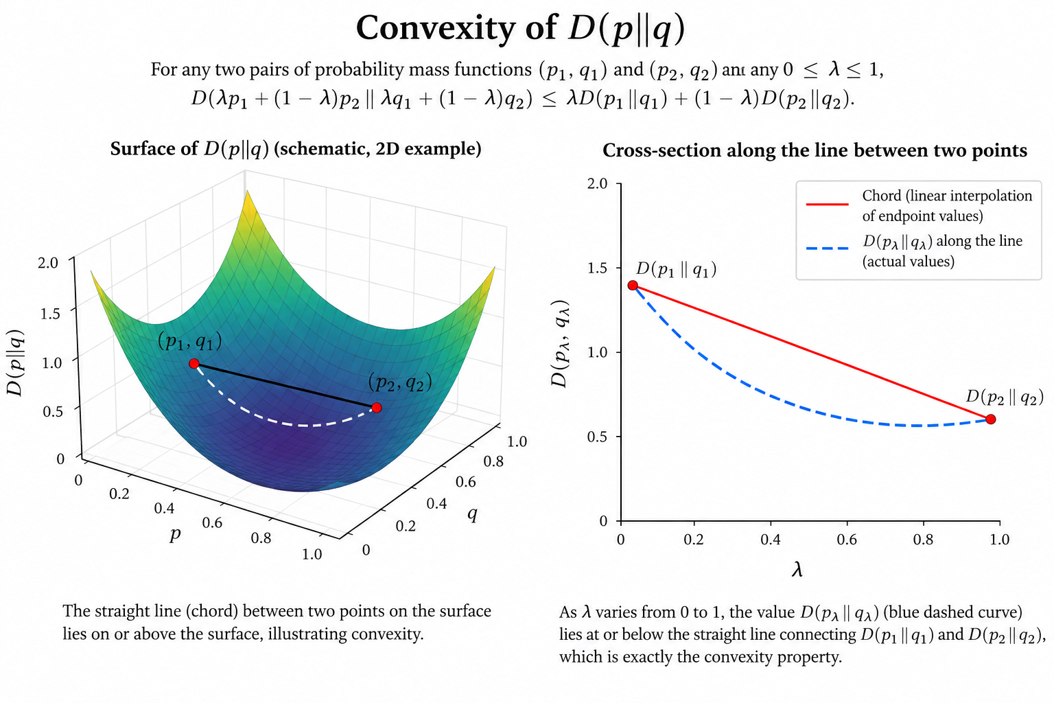 The image above was generated using GPT-5.6 Sol.
Another way to think of this is that mixing and , and and can't make the results more distinguishable than the weighted average distinguishabilities between and and and , i.e., mixing distributions tends to wash out distinctions.
Referenced by (1 direct)
Direct references:
The dot product of and is
where is the angle between and
Referenced by (1 direct)
Direct references:
Let be a cyclic group with elements. Let and . Then generates a cyclic subgroup of containing elements, where . Two cyclic subgroups and are equal if and only if .
Suppose with and let . Then, .
So, .
TODO: Cover & Thomas Theorem 2.8.1.
TODO: Cover & Thomas, corollary to Theorem 2.8.1.
If is the closure of a set in a metric space then
Because
Conversely, Let and such that Therefore, by the triangle inequality,
Therefore, and since was arbitrary,
Referenced by (1 direct, 1 transitive)
Direct references:
Transitive (depth 1):
The directional derivative of in the direction of a unit vector is the inner product of and that is,
Referenced by (1 direct)
Direct references:
Let be a closed bounded region in a space whose boundary is a @piecewise smooth @orientable surface Let be a vector function that is continuous and has continuous first partial derivatives in some domain containing Then
An important theorem related to divergence is the Divergence Theorem (also known as Gauss's theorem) which connects the flux of a vector field through a closed surface to the divergence of the field inside the volume bounded by the surface:
Take a @doubly-stochastic matrix and probability vector let Then with equality iff is a @rearrangement of .
Note that by the definition of vector matrix multiplication. Now we'll define a couple of joint distributions:
Now we find the relative-entropy from to :
Now, addressing the first term on the RHS of the last line:
And the second term on the RHS of the last line:
So, we end up with Since by Gibbs' Inequality, we have which implies that which is what we wanted to show.
Now, the equivalence case. If is just a rearrangement of then obviously it has the same entropy as we can just re-index to recover Now assume Then, whenever Now, for each value appearing in or let
that is is the set of indices of where and similarly with and Now, consider row For any we have so i.e. every nonzero entry of row lies in a column of so the columns have the entire mass of row Similarly, for column for nonzero so and the rows contain all of column 's mass. Taking as the @indicator-vector of a set we have that
that is, rows in sum to over the columns while rows outside have no mass in the columns at all. Now we count the mass:
Therefore, for all so each appears equally often in and in and is therefore a rearrangement of
Averaging (well, replacing each probability with a convex combination of all the probabilities in a way that retains their summing to 1) the probabilities in can only bring them closer to each other (if it doesn't just rearrange them), which increases entropy.
is a metric space for any
First, for , is just the empty set, so the metric axioms are vacuously satisfied for all points in the set. Now, for
- Let Then so
- Let Now, so so
- Let so
- Let so
Therefore, is a metric on and is a metric space.
is separable.
The points of that have only rational coordinates are a subset of we'll call it countable and dense.
We know that the rationals are countable, and because -tuples of countable elements are countable, is countable.
To show is dense, consider an arbitrary point in Now, let Since the the rationals are dense in the reals, we can pick a with by picking rational approximations of the coordinates of and forming such that is within of i.e.
Referenced by (1 direct)
Direct references:
All Euclidean spaces are complete
That is, in every cauchy sequence converges.
Let be a cauchy sequence in Define as in the proof above, but with in place of For some The range (sequence) of is the union of and the finite set Hence, is bounded (sequence) (since the finite set of points can be contained in some bounding box, and the remaining points can be contained in some ball with diameter 1.) Since is bounded, it is compact, and thus is a subset of a compact metric space (its closure), and so converges.
Referenced by (1 direct)
Direct references:
Every convergent sequence in a metric space is a Cauchy sequence.
Suppose is a convergent sequence in a metric space Let Then for some when Thus,
whenever and so is Cauchy.
Referenced by (1 direct)
Direct references:
Every -cell is compact.
Let be a -cell, consisting of all points such that Let i.e., the maximum distance between any two points in (the diagonal). Then for any points
Suppose, for the sake of contradiction, that there is an open cover of that contains no finite subcover of Now, let i.e. is the midpoint of We can subdivide into -cells determined by the intervals and At least one call it cannot be covered by any finite subcollection of or else would have a finite subcover in We then can subdivide and so on, obtaining a sequence with the following properties:
(a) (each -cell in the sequence is nested in the previous.)
(b) is not covered by any finite subset of
(c) If then
From (a) and If is a sequence of intervals..., there is some point that is in every For some since is a cover of all of is open, so for some implies that that is, has a neighborhood that lies entirely within If we make big enough, we have that so by (c), that is, is entirely covered by But, this contradicts (b), so our provisional assumption is incorrect, and must have a finite subcover that covers and therefore is compact.
If a -cell has an open cover , then any point in it will be in some and can therefore be surrounded by an open ball with some positive radius, lying entirely in . That open ball takes up some space, and we can then subdivide the -cell into small enough parts that some part is entirely within that open ball. We still have finitely many subdivisions, and each of those could be covered with a similary constructed open ball, which means we can cover the entire -cell with finitely many open balls covered by finitely many elements of
Referenced by (2 direct)
Direct references:
Let be a metric space in which every infinite subset has a limit point. Then is separable.
Let and pick Now, continue picking such that i.e. so that each new point is at least away from each existing point. Suppose this process continues infinitely; then the points are an infinite subset of and thus must have a limit point Now, because every neighborhood of must contain infinitely many points in , we can let be a neighborhood of and pick But, by the triangle inequality
so which contradicts our assumption that could be an infinite set where all points were at least apart. Therefore, has only finitely many points, and can be covered with finitely many open balls of radius (for if it couldn't be, we could always fit another point into )
Now, if we let we can consider the set of points as the finite set of points at least apart in The collection of all such points can be called and is dense in let be a point in and a neighborhood of If we pick such that then some will be in because if not, we would have a contradiction with the fact that shown above that no point in is more than away from a point in
Since each is finite, and there are countably many the is a countably dense subset of and therefore is separable.
Referenced by (1 direct)
Direct references:
Every neighborhood is an open set.
Suppose is a neighborhood in Let We need to show that is an interior point of Let because , we have Now let be the neighborhood of radius around We need to show that Suppose First note that because Now,
Therefore, so is an interior point of and since was arbitrary, every point of is interior. Hence, is open.
Referenced by (1 direct)
Direct references:
Every separable metric space has a countable base.
Let be a separable metric space, and let with @open-set. Now, because is separable, it by definition has a countable dense subset If we can pick a rational and let be a neighborhood such that ( must also be small enough such that this neighborhood is within which is possible because is an interior point of and we can pick a rational as close to any real as we'd like.) Now we have that and since there are countably many and countably many neighborhoods with rational radius around each there are countably many such neighborhoods in On the other hand, if then is a limit point of and thus there is as close as we'd like to Pick such that for some rational such that Again, since there are countably many such with countably many neighborhoods of rational radius each, there are countably many such neighborhoods in
Now, if we let be the union of all open sets then is open, and let be the union of all the with then every is in some and there are countably many so is a countable base for
Referenced by (2 direct)
Consider the @initial-value-problem
Suppose that and are continuous on an open interval of the -axis, and suppose that is a point in Then, the initial value problem has a solution on some time interval about and the solution is unique.
TODO: Cover & Thomas Theorem 2.10.1.
TODO: Cover & Thomas, Section 2.10.
If is given by then at the tangent plane is
Let and be a positive integer. Then
First, define as
Then
Subtracting the second equation from the first gives
because everything in the middle cancels out.
Now, we can factor out from the left hand side to get
Referenced by (1 direct)
Direct references:
Suppose is a finite set in metric space and that is an open cover of Since is finite, we can enumerate its points as for some Then, for each (there are none when ,) pick an with Define the index set Because is finite, is finite as well, and so is a finite sub-cover of the original open cover. Therefore, every open cover of has a finite sub-cover, and is compact.
Let be a positive integer. Then the vectors
for form a basis for
To show linear independence, we will show a stronger condition, orthogonality, holds.
For we can write that the th entry of is
and that the conjugate of the th entry of is
Then, in our inner product between and , the th term is
Thus, for
Now we need to show that this sum is Note that if we let we can rewrite this as
From Finite Geometric Series, we have that
Substituting back in for we get
Thus, and so when an are orthogonal and therefore @linearly-independent.
Now we need to show that span
Let We need to find such that
That is, we want constants such that
To find some specific we can take the inner product of both sides with respect to to get
@Linearity in the first argument of the inner product allows us to rewrite the right side to get
Now, we know that
so the inner product on the right-hand side is except when and this reduces to
Therefore,
This shows that the Fourier basis described here indeed spans and shows how to compute the Fourier coefficients
Suppose and are metric spaces, with a limit point of and Then, is continuous if and only if
Note that the definition of a function having a limit at point in a metric space is different from the definition of a function being continuous at a point in a metric space only in that the continuous definition requires the function to be defined at the point (and equal to the limit at the point.)
When a line integral is known to be independent of path, and its value is required along some curve with initial point and final point , we can either replace the given curve with a simpler curve, or, take the difference in the values of the function at and .
For discrete probability distributions and that share a support
with equality iff Equivalently, cross-entropy is never less than entropy: with equality iff
Because Log is Concave, by Jensen's Inequality we have that
Then, since we have that
Now, note that if and Conversely, suppose Since is strictly concave, it is not @affine, and Jensen's Inequality condition for equality gives us that Now, and since is a probability distribution, and therefore and
For any two random variables, with equality if and only if and are independent.
Using the definition of mutual information and Gibbs' Inequality, we have with equality if and only if i.e. and are independent.
with equality if and only if for all and such that
From the definition of conditional relative entropy we have
This is just the average of the relative-entropy over distributions over for each fixed For each is if and only if by Gibbs' Inequality, and positive otherwise.
with equality if and only if and are conditionally independent given
We have that
and for each fixed
.
By Gibbs' Inequality, the quantity for each fixed is non-negative, so the sum weighted by the probability of each is also non-negative.
For equality, the average is if and only if for each with
why by Gibbs' Inequality means
for all i.e. and are conditionally independent given
Gradient fields are irrotational. That is, if a continuously differentiable vector function is the gradient of a scalar function then its curl is the zero vector:
Furthermore, the divergence of the curl of a twice continuously differentiable vector function is zero:
Let be a differentiable scalar function in space. Let (with constant) represent a surface Then, if the gradient of at a point of is not the zero vector, it is a surface normal vector of at
Any curve lying in can be parameterized as such that
Now, if we differentiate (a) with respect to we get
Therefore, is orthogonal to all the vectors in the tangent plane of at and is therefore a surface normal vector of at
The force of attraction
between two particles at points and (as given by Newton's law of gravitation) has the potential function where is the distance between and
Thus, This potential function is a solution of Laplace's Equation
that is, has a Laplacian of
Suppose and have continuous first partial derivatives in a domain containing a simple, closed, piecewise smooth curve and its interior Then
Referenced by (2 direct)
Direct references:
If a set in has one of the following three properties, then it has the other two:
(b) is compact.
(c) Every infinite subset of has a limit point in
If (a) holds, then for some -cell and (b) follows from the facts that every -cell is compact and closed subsets of compact sets are compact. Then, (c) follows from the fact that any infinite subset of a compact set has a limit point in . To complete the cycle of implication, we must now show that (c) implies (a).
Assume, for the sake of contradiction, that is not bounded. Then, must contain an indexed set of points where each must satisfy is obviously infinite, but we will show it has no limit points in Let Then for some positive integer Since is finite, there can only be finitely many points in with If is empty, then is obviously not a limit point of Otherwise, let Then and let be a neighborhood of Since no point in other than perhaps lies in is clearly not a limit point of Thus, our provisional assumption is invalid and (c) implies is bounded.
To show that (c) implies is closed, assume for the sake of contradiction that is not closed. Then, there is a point which is a limit point of but is not in We will construct an infinite subset of and show that it has no limit point in For let the point be some point in such that let be the set of such points. is certainly infinite, because will eventually be bigger than for some if we keep reusing the same infinitely many times. Now, has as a limit point, and we will show it is its only limit point in Assume Then, via the triangle inequality, for all but finitely many and thus is not a limit point of because its its neighborhoods do not contain infinitely many points of . Thus, has no limit point in which contradicts (c), and therefore our provisional assumption that is not closed is incorrect, and (c) implies that is closed.
Without proof here, (b) and (c) are equivalent in any metric space, but (a) does not imply (b) and (c) in every metric space (we assumed above.)
Referenced by (4 direct)
One useful fact you may recall from linear algebra that also applies with group homomorphisms is that is injective iff the kernel of is .
Let be a metric space in which every infinite subset has a limit point. Then is compact.
By Let be a metric space in..., we know that is separable and by Every separable metric space has a countable..., we know that has a countable base. By the definition of base, we have that every open cover of has a countable subcover
Suppose, for the sake of contradiction, that has no finite subcollection that covers Let
Then, each must be nonempty (otherwise a finite subcollection of would cover However, since every point in is in some
Now, let be a set with a point from each Since there are infinitely many is an infinite subset of and therefore has a limit point, Now, must be in some open and so for some
Now, note that each because is formed by excluding all the points in that are also in Because is a limit point of must contain infinitely many points of However, only finitely many points of can be in because for contains no points in Therefore, is not a limit point of and no such limit point can exist, contradicting our hypothesis that every infinite subset of has a limit point. Therefore, must be finite, and must have a finite subcollection that covers meaning is compact.
If is an infinite subset of a compact set then has a limit point in
Assume, for the sake of contradiction, that no point in is a limit point of Then any point in has a neighborhood with at most one point in if Since is infinite, an infinite number of these singleton neighborhoods would be required to cover it, and therefore to cover since But, this contradicts our hypothesis that is compact. Therefore, our provisional assumption must be false, and must contain a limit point of
Referenced by (3 direct)
Every infinite subset of a countably infinite set is countable.
Assume is countably infinite, and Arrange a sequence from the distinct elements of . Let be the smallest positive integer such that and then pick by assigning the next in the sequence the index of the left-most entry in that has not yet been picked. Then, let be the smallest integer greater than such that Now, is a sequence of strictly increasing positive integers giving us the indices of the first elements of in
Now, define as , which is a bijection between the positive integers and , showing that is countable.
We can show this by putting into a sequence of distinct values, so it can be indexed with the positive integers, and then constructing a subsequence of that are only the indices of elements of
As an example, consider the even numbers as a subset of the non-negative integers Then, the indices of the even numbers are and
This means that countably infinite sets are the smallest infinite sets. Any infinite subset of one has the same cardinal number as the parent set, and the same cardinal number as the set of natural numbers - - "aleph null."
If is the unit circle, then
First, note that we can parameterize the unit circle, as
Now, making the substitution,
Now, using the definition of the contour integral,
we have, noting that
Referenced by (1 direct)
Direct references:
If is a sequence of intervals in such that then is not empty.
Let and let be the set of all Then, is nonempty, because even if for all it at least contains a single point. It is also bounded above by since any is in Let Let and be positive integers and we have that so that for each Since we have that that is, for all so and thus is not empty.
Referenced by (1 direct)
Direct references:
Let be a random variable with finite expectation , and let be a convex function. Then
If is concave, the inequality reverses:
In either case, equality holds if and only if is @affine on the support of , or is almost surely constant.
We will proceed by induction. Assume is discrete and takes on values with probabilities
Base step, for : Assume takes on two distinct values, and with probabilities Then we want to show that
The last line is just the definition of a convex function, so it's obviously true.
Inductive step: Assume that (a) holds for any points. Take points with weights summing to Let
Assuming let Then, so the form an -point distribution. Now, we'll rewrite to bundle the first terms separately from the last term:
where Now, because (b) is a two-point convex combination of and From our base case,
Now, from our inductive hypothesis we have that
Tying it all together we have
TODO: show the equality case only holds when the support is affine.
Referenced by (3 direct)
Let and be discrete random variables with alphabets and and let be the probability of the joint occurrence of and
The entropy of the joint event (the joint entropy), is less than or equal to the sum of the individual entropies, i.e.
with equality iff and are independent, that is, iff
The entropy of the joint event is
This is just treating each possible pair of individual outcomes as its own outcome, i.e. we have possible outcomes. Writing and for the marginals (the argument names the distribution), we have
So,
Now, let's define a new random variable for convenience, We now have that
Now, by Jensen's Inequality, because Log is Concave, we have that Now,
Therefore and we have that and
Now, for the equality part. Suppose Then, and recalling that In Jensen's Inequality, equality holds only if our function is @affine or if is constant; since is @affine on no interval, must be constant, and since
Now, suppose Then and
so
Referenced by (1 direct)
Direct references:
Suppose and are subgroups of a group such that and suppose that and are both finite. Then is finite.
The intuition here is that each coset of can be partitioned into cosets of , and that can be partitioned into cosets of , so can be partitioned into cosets of . Since both and are given as finite, their product is also finite.
In more detail, say can be partitioned into cosets of , where is a natural number. Let be a set of coset representatives such that is a partition of formed by the left cosets of .
Then, is
and each is a disjoint coset of in .
Now, can be partitioned into cosets of , where is a natural number. Let be a set of coset representatives such that is a partition of formed by the left cosets of .
Then, . Now, we can recover by taking the union of the elements of , that is, , so the elements of , after a round of flattening, are the same as those of If we replace in (a) with , distribute each group action over the elements of , and then take the union across each resulting set we end up with
which is partitioned into the left cosets of . Because we constructed each element in by partitioning the elements of a partition of into cosets of (then taking their union), we know they are disjoint and cover all of . There are elements in , and since and are finite, so is .
If is the proportion of successes in a random sample of size and an approximate confidence interval for the binomial parameter is given by
When is small and the unknown proportion is believed to be close to or , this approach doesn't work well and shouldn't be used. This approach should only be used when both and are greater than or equal to
Suppose are independent and identically distributed random variables with finite @mean Then for any
Intuitively, this means that the more identically distributed random variables we have, the closer their average value will get to the mean for the random variables. If we think of each random variable as an identical sample from the same population, another way to think of this is the more samples we get, the closer the average value across all samples will be to the true average value for the population, and we can get as close as we like to the true average value for the population by taking more samples.
We assume that the variance of the random variables is also finite. Then, note that
and
Then, by Chebyshev's Inequality, we have
Now, as increases, the term on the right approaches , which by the Squeeze Theorem implies the term on the left also approaches and is at the limit.
Let and be metric spaces; suppose and is a limit point of Then
if and only if
for every sequence in such that
Suppose that (a) is true and let be a sequence such that (c) holds. Let Then, for some if then Now, there is also some such that whenever and thus, whenever so (b) holds.
Conversely, suppose that (a) is false. Then, for some that for every there exists a point such that but If we let and each a point such that then is a sequence satisfying (c). However, since for all (b) does not hold.
If has a limit at this limit is unique.
This follows directly from the facts that limits of sequences are unique and that limits of functions are characterized by limits of sequences.
Referenced by (2 direct)
if is a sequence in and if consists of the points then is a Cauchy sequence if and only if
Suppose is a Cauchy sequence. Then, let For some integer when Therefore, Since was arbitrary, we can see that the sequence converges to
Conversely, suppose Then, every neighborhood of contains for all but finitely many N. Let Then, pick such that Letting we have that
Referenced by (1 direct, 1 transitive)
Direct references:
Transitive (depth 1):
If and if is a limit point of then there is a sequence in such that
For each there is a point such that . Let and pick so that Then, if so .
Let be the set of all limit points of a set in space Then is closed.
Let Then some neighborhood of contains no points in other than possibly itself. If contains only then is not a limit point of Suppose, for the sake of contradiction, some point is a limit point of Then, every neighborhood of contains some point in Let be such a neighborhood, and let be a limit point of . Now, has neighborhoods wholly in and such neighborhoods can have no point in so we have a contradiction, and therefore is not a limit point of Hence, is an interior point of and is open, and therefore is closed.
If and converges to and then
Suppose, for contradiction, that Then, Let and be balls around and respectively. This means that only finitely many points from are not in . However, since and are disjoint by construction, this means only finitely many points of are in a contradiction. Therefore, our assumption that is incorrect, so
Referenced by (2 direct)
If is a continuous function of two variables whose domain includes the smooth curve , then the line integral can be evaluated as:
Let be a fixed point of Then, if if is negative, then is a stable fixed point . If is positive, then is an unstable fixed point.
This comes from letting be a small perturbation away from differentiating it, writing its taylor series, then noticing that and terms greater than the linear term matter less than the linear term and writing
This is called the linearization about
It also only works if If that's not the case, the best bet is to fall back to graphical analysis or to solve explicitly if possible.
The function is concave, i.e. is convex.
The second derivative of natural is which is always non-positive. By Second Derivative Test for Convexity, is therefore concave.
Referenced by (2 direct)
For non-negative numbers, and
with equality if and only if
We use the conventions that if and all of which follow from @continuity.
We can assume without loss of generality, due to the -handling conventions specified above, that and Now, note that the function is @strictly convex, since for all positive Then, by Jensen's Inequality we have
as long as i.e. if the form a @discrete probability distribution.
If we let , i.e. is the @probability mass assigned to index then this condition is met. We can then pick and we get
Referenced by (2 direct)
By definition,
Referenced by (1 direct)
Direct references:
A mapping of a metric space into a metric space is continuous on X if and only if is open in for every open set in (see inverse image.)
Assume is continuous on and is an open set in Suppose, for the sake of contradiction, that is not open. Then, some point is not an interior point of which means there is no neighborhood of that contains only points in that is, every neighborhood of contains some point that is not in i.e., Now, since is open and there is some for which but, since all neighborhoods of contain some there is no for which all points within of are mapped to by a contradiction, since is continuous on by hypothesis. Therefore, our assumption is incorrect and is open.
Conversely, suppose is open in for every open set in Let be an open set in Assume, for the sake of contradiction that there is some at which is not continuous. Let Then, there is no for which contains only points that are mapped by to i.e. every neighborhood of contains some point that is not in and therefore is not an interior point of and is not open, a contradiction. Thus, our assumption must be incorrect, and there is no such and since entire space is an open subset of itself, must be continuous on all of
A mapping of a metric space into a metric space is continuous on if and only if is closed in for every closed set in
First, note that for any we have since exactly when which is exactly when
Now, as ranges over the open subsets of its complement ranges over the closed subsets of by A set is open iff its.... So, by A mapping of a metric space..., is continuous on if and only if is open in for every closed set in By the observation above, and this is open in if and only if is closed in again by A set is open iff its....
Referenced by (1 direct)
Direct references:
Referenced by (1 direct)
Direct references:
Let be a non-negative random variable () and Then,
That is, the probability that is at least has an upper-bound of the expectation (mean) of divided by In simpler terms, the probability that can't be too big.
Note that as grows larger, the probability of being greater than grows smaller.
This follows from the Law of Total Expectation, which is
Here, we're partitioning 's sample space into a portion above and a portion below
Now, is the expected value when which is necessarily at least since is restricted to taking on values of at least So, we have that
We can substitute this into (a) to get
Note that our equation has turned into an inequality; we must do this because the original RHS was equal to the original LHS, and the original RHS is greater than or equal to our new RHS, which means the original LHS is greater than or equal to our new RHS.
Now, since we said that is non-negative, its expected value is also non-negative, including when We have by definition that is non-negative (because all probabilities are non-negative). Therefore, must also be non-negative as it's the product of two non-negative numbers. Since the LHS of (b) is greater than the RHS with this non-negative value added to the RHS, the LHS is also bigger without it added, and therefore we can drop it to get
Dividing both sides by and swapping sides gives us
Referenced by (3 direct)
Suppose is continuous on and differentiable on Then there exists a point in such that:
This means that for a function continuous on an interval, and differentiable on that interval except maybe at its endpoints, there is a point on the interval where the derivative of the function at that point equals the slope of the function between its endpoints.
The moment generating function for the sum of two random variables is the product of the moment generating functions of the two random variables. More generally, if are independent random variables, then
We'll prove the case where the general proof is exactly the same but more tedious.
TODO: state and the -variable chain rule Note it reduces to a product distribution when the variables are independent.
TODO: rearrange the definition of conditional probability distribution; induct for the -variable form.
Referenced by (1 direct)
Direct references:
We'll prove (c) first:
Now, from Chain rule for joint entropy we prove (a) and (b) with
and
(d) is trivial from symmetry of and
To prove (e) we use our result from (a):
Referenced by (1 direct)
Direct references:
Let be a countable set, and let be the set of all -tuples where and the elements need not be distinct. Then is countable.
We will proceed using proof by induction. First, for the base case, note that is the set of -tuples formed by elements of , so and is thus countable. Now, for the inductive step, assume is countable Then we have that
So, for any given -tuple , we form -tuples by appending each element of to it, and so the set of pairs has the same cardinality as and is thus countable. is thus the union of the countable set of countable sets (the set of sets formed by appending each element of to each element of ) and is therefore countable itself, by a theorem proved above. Therefore, by induction, every is countable.
The set of rational numbers is countable.
Rational numbers just formed from pairs of integers: so we use the above theorem with
Referenced by (2 direct)
Referenced by (1 direct)
Direct references:
The negation of a conjunction is the disjunction of negations.
Let and be boolean variables. We want to show that
First, assume is true. Then, both must be false, so either must be false or must be false, or both must be false. If is false, then is true, and so is The same is true if is false, so
Now, assume is true. Then, either or must be true, so either or or both must be false. Now, if is false, then is false. The same holds if is false, and thus is true. Therefore and we have shown
The negation of a disjunction is the conjunction of negations.
Let and be boolean variables. We want to show that
First, assume is true. Then, is false. If were true, then we'd have a contradiction, and similarly with so both and must be false, that is, and most both be true, and
Now, assume Here, both and must be true, so both and must be false. Therefore, is false, so and we have shown
If is a limit point of a set then every neighborhood of contains infinitely many points of
Let be a limit point of and let be a neighborhood of Suppose that contains only finitely many points of Since we have finitely many points, we can inspect each and find the minimum distance from to any point in and call it Now, we can make a new neighborhood which contains none of the points in since they're all at least away from by construction. But then, is not a limit point of since it has a neighborhood that contains no points of Therefore, we have a contradiction, and must therefore contain infinitely many points.
From this, it's evident that a finite set of points has no limit points. That is, if a set has a limit point, then the set if infinite.
Referenced by (2 direct)
If is a sequence of nonempty compact sets in such that and if
then consists of exactly one point.
Let Then is not empty. Assume for the sake of contradiction that contains more than one point. Then, But, for each so that But, this contradicts our given that so our assumption that contains more than one point must be invalid, and thus contains exactly one point.
Referenced by (1 direct, 1 transitive)
Direct references:
Transitive (depth 1):
Given a communication channel which has a capacity of bits per second, accepting signals from a source of entropy (or information) of bits per symbols, it is possible, given a properly devised coding procedure, for the transmitter to transmit symbols over the channel at an average rate which is nearly but which, no matter how clever the coding, can never exceed
Let be a nonempty perfect set in Then is uncountable.
We know that is infinite, because by definition, all points in perfect sets are limit points, and only infinite sets have limit points.
Suppose, for the sake of contradiction, that is countable. Label the points of as We will construct a sequence of of neighborhoods.
As a base step, let be any neighborhood of let (note: subsequent aren't required to be neighborhoods of ) Then the closure of is
For the inductive step, suppose as an induction hypothesis that we have some that's been constructed such that is not empty. Since every point of is a limit point of we can make a neighborhood such that (i) (ii) (iii) is not empty. Now, satisfies our induction hypothesis, and since does too, we have defined for all
For each , let Since is closed and bounded, is compact. Since no point of lies in Since this implies that is empty. But, each is nonempty, by (iii), and , by (i). But the intersection of nonempty compact nested sets is nonempty, so we have a contradiction, so our provisional assumption that is countable must be incorrect. Therefore, is uncountable.
Every interval is uncountable, and thus the set of all real numbers is uncountable as it contains uncountable subsets.
Referenced by (1 direct)
Direct references:
Referenced by (2 direct)
If is a collection of compact subsets of a metric space such that the intersection of every finite subcollection of is nonempty, then is nonempty.
Let for each and note that since is compact and therefore closed, is open. Then, fix a member of Assume, for contradiction's sake, that no point of is in all that is, that Then, any point is in some so forms an open cover of Since is compact, some finite subset of forms a finite subcover of such that (by De Morgan's.) Therefore This is an empty intersection of a finite subcollection of which contradicts our hypothesis that all finite intersections are nonempty. Therefore, our assumption that no point in is in all is incorrect, and some point in is in all and therefore is not empty.
If is a sequence of nonempty compact sets such that then is not empty.
Suppose Then, by definition, and by induction, Then, every is a nonempty subset of and so the intersection of any finite number of these will be nonempty, and by If is a collection of compact..., is not empty.
Referenced by (2 direct)
Referenced by (1 direct)
Direct references:
For discrete probability distributions and that share a support
with equality if and only if
This restates Gibbs' Inequality, which the Log Sum Inequality proves more directly.
with equality if and only if Both and are probability mass functions, so (otherwise they wouldn't both sum to 1) and hence we have if and only if for all
If is a binomial random variable with mean and variance then
This works well when is large and is not extremely close to or , and also works well when is small and is near
Let be a binomial random variable with parameters and For large , has approximately a normal distribution with and and
and the approximation is good if and are greater than or equal to 5.
The is called a continuity correction and comes from the fact that
For complex and integer with we have
A set is open iff its complement is closed.
First, consider the case that is empty, and therefore open. If has no limit points, it is vacuously closed. Suppose has a limit point Since is empty, must be in therefore is closed. Now, consider the case that is empty, and therefore closed. If is empty, it is open, and the theorem is satisfied. If is not empty, a point in has only points in in any neighborhood, since all points are in and therefore is open.
Now we deal with the cases where neither nor are empty.
Now, let be closed. Let Since is closed, is not a limit point of that is has some neighborhood that doesn't contain a point in and must therefore be a subset of Therefore, is an interior point of and is open.
Conversely, assume is open. Let be a limit point of Suppose, for the sake of contradiction, that Then, since is open, is an interior point of and has some neighborhood that is a subset of This is a contradiction, since every neighborhood of must contain at least one point of to be a limit point of Therefore, must be in and it follows that is closed.
Suppose A subset of is open relative to iff for some open subset of
Suppose is open relative to Then, for every there is some such that implies that Let be the set of all where (and thus ) and let
Then, since each is an open subset of so is Now, since for each Also, since for every and
Conversely, suppose for some open subset of Now, suppose Then, and there is some neighborhood Then, so is open relative to
Referenced by (1 direct)
Direct references:
Every open set in is the union of an at most countable union of disjoint segments.
Let be an open set in Let Let and Then, because is open and thus is an interior point of and there is some neighborhood around that is entirely within Let By construction, is connected. For all must have the same end points as since if it extended beyond, our construction of would be contradicted. Also note that for all for if they intersected, they would form an open interval. Thus, each is either disjoint from all others or identical to some other and is the union of all such unique
Now, in each we can pick a rational number. Because the rationals are countable, we have at most countably many unique and is their union.
Every permutation of a finite set is a product of disjoint cycles.
A permutation in can be written as either a product of an odd number of transpositions or a product of an even number of transpositions, but not both.
Let be a nonempty set, and be the collection of all permutations of . Then is a group under permutation multiplication.
Suppose that
(1) is a closed, bounded subset of the plane;
(2) is a continuously differentiable vector field on an @open-set containing
(3) does not contain any fixed points;
(4) There exists a trajectory that is "confined" in in the sense that it starts in and stays in for all future time.
Then, either is a closed orbit, or it spirals toward a closed orbit as In either case, contains a closed orbit.
Referenced by (1 direct)
Direct references:
Let be a binomial random variable with probability distribution When and remains constant,
TODO: the log of a power moves the exponent out front.
The set of probability vectors in is a convex set, and it is compact.
Let be the set of probability vectors in That is,
(Note: is a dimensional @simplex).
Suppose Then
.
Then, let Now,
Since either or are non-negative, all entries of this convex combination are non-negative, so the combination is again in and is therefore a probability vector.
We can use Heine-Borel to show that is compact by showing it is closed and bounded.
Noe that for each and each @coordinate
is a closed half-space. Now, note that the map
is continuous, the pre-image of under is
Because is closed in by A mapping of a metric space... we have that
is closed
Now,
is an intersection of closed sets, which is also closed.
is obviously bounded - the sum of all coordinates in is always so the closed ball of radius centered at the origin.
Therefore, is closed and bounded, and is compact.
TODO: we can generalize this to the fact that @simplexes are convex and compact.
Referenced by (1 direct)
Direct references:
TODO: the log of a product is the sum of the logs.
Referenced by (1 direct)
Direct references:
Referenced by (1 direct)
Direct references:
TODO: the log of a quotient is the difference of the logs.
The radius of convergence of the Taylor series for a function about a point is the distance from to the nearest singularity of .
The rationals are dense in the reals.
Let and Pick such that Now, because the reals are Archimedean, for some we have that Then,
Now, if we let we have
so Therefore, every neighborhood of contains some and so is either a limit point of or else and so the rationals are therefore dense in the reals.
If and then there exists a such that That is, there is always a rational number between any two distinct real numbers.
Pick such that Because because the reals are Archimedean, there is some such that and Thus, and
Let be analytic inside a simple closed path and on except for finitely many @singular-points inside Then,
Referenced by (1 direct)
Direct references:
If is used as an estimate of we can be confident that the error will not exceed a specified amount when the sample size is
If is used as an estimate of we can be confident that the error will be less than a specified amount when the sample size is approximately
Let be twice differentiable on an open interval Then is convex on if and only if for all and concave if and only if for all
Referenced by (1 direct)
Direct references:
converges to if and only if every neighborhood of contains for all but finitely many
Suppose converges to Let For some integer when Therefore, for all but the finitely many where
Conversely, suppose every neighborhood of contains all but finitely many i.e., for all but elements of Let Then, whenever therefore,
Referenced by (3 direct)
If is a sequence in a compact metric space then some subsequence of converges to a point in
Let be the range of If is finite, then at least one point in must be repeated infinitely many times in If we let be the indices of the occurrences of in
then the subsequence converges to
On the other hand, if is infinite, then has a limit point . Pick so that Now, after picking we can pick such that , so converges to
Referenced by (1 direct)
Direct references:
If is a set in a metric space, then and have the same limit points.
If is closed, then we are done, because a set equals its closure if it is closed.
Suppose is a limit point of Then every neighborhood of contains some Since , so is a limit point of
Conversely, suppose is a limit point of Then, every neighborhood of contains a point of If then clearly contains a point in Otherwise, Now, since and every neighborhood is an open set, has some neighborhood Since contains some point Since and therefore contains a point in Thus, all neighborhoods of contain some point in and is a limit point of
A set and its limit points do not necessarily have the same limit points.
Consider Then has one limit point, but has no limit points, since the only number that contains in all its neighborhoods is itself (see From this, it's evident that a finite....)
If is a metric space and then
(a) is closed.
(b) iff is closed.
(c) for every closed set such that
By (a) and (c), is the smallest closed subset of that contains
(a) Suppose and Then is not in and is not in and is in fact in Now, since is not a limit point of it has some neighborhood that does not intersect Any point in is an interior point of , and therefore has its own neighborhood that does not intersect and therefore is not a limit point of Thus, any point in is an interior point of and is therefore open and its complement, is closed (since a set is open iff its complement is closed.)
(b) Suppose is closed. Then it contains its limit points, so Conversely, suppose By (a), is closed.
(c) Suppose that and that is closed. Suppose If then because If then it must be in also, since contains all points of and is closed, and thus must contain the limit points of
Referenced by (2 direct, 1 transitive)
Direct references:
Transitive (depth 1):
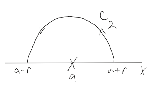
If where each is a closed subset of then at least one has a non-empty interior. Equivalently, If is a dense open subset of for then is not empty (in fact, it is dense in .)
First, note that since every point in is in some and so must be empty.
Suppose, for the sake of contradiction, that no has a non-empty interior, that is, every is closed with an empty interior. Then, each is open. Moreover, since has an empty interior, it has no points for which there exists a neighborhood that contains only points in that is, every neighborhood of each point of contains a point in so every point in is a limit point of and every point in is either in or is a limit point of so each is non-empty and dense in
As a base step, let be some point in and let be an open ball around Since the interior of is empty, is not empty, and is open.
For the inductive step, suppose we have some that's constructed such that is non-empty and open. Then, we can pick a point and make a ball around it such that and is open and not empty. Now, since satisfies our induction hypothesis, and since does as well, we have defined for all
Since the set of points is infinite (by induction) and bounded (all points are within ,) it has a limit point in . Now, suppose, for contradiction, that is not in every Then, for some is not in Since and , we have . Since is open and is outside it, is at some positive distance from any point . But for all , so all these infinitely many points are at distance at least from . Thus any neighborhood of with radius less than contains at most finitely many points of , contradicting that is a limit point.
Now, this means that meaning a contradiction! Therefore, our supposition that every has an empty interior must be incorrect, and some must have a non-empty interior.
When the markov chain is ergodic, the limit
exists and
Here, and the entries in it represent the long term probabilities of being in any given state, or equivalently, the portion of time spent in any given state.
Note that which when combined with the fact that the entries of sum to 1 lets us solve a linear system of equations to find the entries of
Referenced by (1 direct)
Direct references:
Let be a @piecewise smooth oriented surface in space and let the boundary of be a piecewise smooth simple closed curve Let be a continuous vector function that has continuous first partial derivatives in a domain in space containing Then
Here is a unit @normal-vector of is the unit tangent vector and the arc length of
In components, (2) becomes
Here, and is the region with boundary curve in the -plane corresponding to represented by
Start with a source of states emitted by a @stationary ergodic Markov chain with transition probabilities and Stationary Distribution of an Ergodic Chain . Its entropy rate is, by definition, A message is a sequence of length each . Such a message is a path through the network with probability Let Then there exists such that for all the length- sequences split into two classes:
- The typical set,
- The atypical set, with total probability
Moreover the convergence holds @almost surely: so with probability a drawn sequence is typical for all sufficiently large
--- the left eigenvector solving for the transition matrix (eigenvalue normalized so ).
The subsequential limits of a sequence in a metric space form a closed set subset of
Let be the set of all subsequential limits of and let be a limit point of We want to show that
First, note that if the range of is just then is the only subsequential limit of In this case, is a singleton and is closed set, as it vacuously contains all of its limit points. So, assume this is not the case.
Choose so that and let Suppose are chosen. Since is a limit point of there is an with Since and is thus the limit (sequence) of some subsequence of there is an such that Now, via the triangle inequality,
This means that converges to because we can find a as close as desired to Therefore is a subsequential limit of and so and is closed.
Referenced by (1 direct)
Direct references:
Sum of cubes:
Difference of cubes:
If are independent normal random variables with means and variances then the random variable is normal with mean and variance
If are independent Poisson random variables with parameters then is a Poisson random variable with parameter
Suppose and are complex sequences, and Then
(a)
(b) for any number
(c) for any number
(d)
(e)
For (a), let pick such that when and pick such that when Then, let Then, when
For (b), If let and then Otherwise,
Let For some when we have
For (c), let For some when we have
For (d), first note the identity
Now, let Pick such that when and pick such that when Then, let Then, when
which means
Applying this, along with the results of (a) and (b) to (1) gives:
For (e), pick such that when so we have that
Now, let For some integer when we have that
Thus, when
Referenced by (1 direct)
Direct references:
Let be a nonempty set of real numbers which is bounded above. Let Then Hence if is closed.
Suppose Then Suppose Now, by hypothesis, for every there is some such that because otherwise, would be an upper bound on Therefore, every neighborhood contains some and thus is a limit point of and
Referenced by (1 direct)
Direct references:
Let be analytic in a domain and be a point in . Then can be expanded in a power series
valid in all circles containing only points of .
If a function can be expressed in the form
valid in some circle , where is analytic at and , then has a zero of order at .
We can see this from the definition of the taylor series. Assume we're at a zero, that is, that Then
and since is we're left with all terms that have in them, and so we can factor them out and get
Now, if does not have a zero at , then is not zero and has a first order zero at If has a zero at we can repeat and move onto the next term until, going through terms, until we find a term that doesn't have a zero at in which case we will have factored out and we'll be left with an analytic with
First we just write the definition:
Now we move the outer exponential into the inner integral, which is allowed since it's constant in :
Now we swap the order if integration. We do this in calc 3... some justify it with Fubini's theorem, it's not clear exactly why this is allowed but this is how it goes (TODO: figure this out)
Now pull out from the inner integral since it's a constant in
The inner integral is just a delta function:
Now by, the sifting property of the delta function, this just reduces to
The th roots of unity under multiplication are isomorphic to under addition.
Let
be the th roots of unity, and
be the first non-negative integers under addition modulo
Let
be a mapping we will show to be an isomorphism.
First, note that and are obviously the same cardinality, by their definitions.
Now, suppose Then
so is a @group-homomorphism.
Now, is 1, that is, so But, is and so is @injective, and an @isomorphism, and and are isomorphic.
The only satisfying the three required properties above is the entropy function defined above, up to multiplication by a constant.
Assume we have a function that satisfies the three properties listed above, such that
Then, by property (3) above, we can decompose a choice from equally likely possibilities into a sequence of choices each from equally likely possibilities. For example, if we have equally likely possibilities, the probability of any given event is . If we instead we have a series of choices each with probability, we end up with as the probability of any specific sequence of events. So, we have that
Now, with arbitrarily large we can also have such that by the same logic, and we can pick such that
Now, we can take the logarithm of each term to get
and dividing by gives
and because is arbitrarily large,
where is arbitrarily small.
By property (2) of (it is a @monotonically-increasing function of ,)
Then, dividing by gives
Now, by the @triangle-inequality, we have that
Since can be arbitrarily small, we have that with so that property (2) holds. Now we know what is, and thus what is when we have equal probabilities for all events.
Now let's say that we have a choice from possible events with commensurable probabilities We can break down a choice from possibilities into a choice from possibilities with probabilities and then, if the th possibility was chosen, choices of equal probability We do this because above, we found how to find when all events are equally likely, and property (3) of our desired function lets us break down our overall choice from possibilities. This gives us
Then,
If the are incommensurable, we can approximate them as closely as we'd like with rationals, since The rationals are dense in the reals.. By the first property we assumed for it is continuous in the and so its value at the incommensurable equals its limit as we approach via the rationals, and so our expression holds in general. is left to us to pick, picking it is equivalent to picking a base for the logarithm.
Pairwise independence is strictly weaker than mutual independence.
When a random variable is uniformly distributed over an alphabet of elements, the self-information of any given element equals the entropy of the random variable and is
If a system has a liapunov function, then its fixed point is globally asymptotically stable: for all initial conditions, as Therefore, the system has no closed orbits.
Like gradient systems, we can't get in a loop if we're always moving downhill.
Let be a scalar function having continuous first partial derivatives in some domain in space. Then, exists in and is a vector, that is, its length and direction are independent of the particular choice of Cartesian coordinates. If at some point it has the direction of maximum increase of at
The directional derivative of in the direction of some unit vector is
where is the angle between and (see The directional derivative of in the... and The dot product of and ...). Note that is a scalar function, as is the directional derivative of Now, has its maximum value of whenever and since is a unit vector with magnitude of 1, (a) simplifies to
which tells us that that direction and magnitude of are independent of the coordinate system chosen. Now, since if and only if and are parallel, is the direction of maximum increase of at assuming at
Let be a continuously differentiable vector field defined on a @simply-connected subset of the @plane. If there exists a continuously differentiable, @real-valued function such that has one sign throughout then there are no closed orbits lying entirely in
iff all the but one are zero, this one having the value of one.
Suppose Then, Note that because we have and (with the convention since ). Assume for contradiction that more than one is non-zero. Then, because each non-zero is in and therefore its and the sum of these terms is therefore non-zero, a contradiction. Now, since all probabilities are required to sum to 1, it can't be the case that all probabilities are zero, which means that exactly one probability must be non-zero and that probability must be
A sequence converges to if and only if every subsequence of converges to
Suppose that converges to Suppose some subsequence converges to and suppose, for contradiction, that Now, following an argument similar to the proof that limits of sequences are unique, we can see that if arbitrary neighborhoods around both can't contain all but finitely many points, so we have a contradiction, and
Conversely, suppose every subsequence of converges to Then, is a subsequence of itself, so it converges to
Due to the magic of linear algebra, if we have a row vector representing the probability of starting in each state, we can compute the probability of ending up in any given state after steps as
Let be the duration of the -th symbol which is allowable in state and leads to state Then the channel-capacity is equal to where is the largest real root of the @determinantal-equation
where is the @Kronecker-delta.
Every closed subset of a complete metric space is complete.
Let be a cauchy sequence. Then, it converges to some point and actually because is closed. Therefore, is complete.
The uncertainty of is never increased by knowledge of It will be decreased unless and are independent events, in which case it is not changed.
From Let and be discrete random... and Chain rule for joint entropy, we have
hence
Suppose a metric space, is a limit point of and are complex functions on and
Then:
This follows directly from the that limits of functions are characterized by limits of sequences, and the algebraic properties of sequences of limits.
If and map into then (a) remains true, and (b) becomes
That is, the limit of an inner product of vector valued functions is the inner product of their limits.
If is a simple, closed, piecewise smooth curve and is interior to , then:
See If is the unit circle, then... and consider path independence and the principle of path deformation. Consider toy contours, particularly a collapsed keyhole contour around the singularity.
Every power series representation of (or, Taylor series for) an entire-function has an infinite radius of convergence.
For any Hamiltonian system, is a conserved quantity.
Random variables are mutually independent exactly when their joint distribution is a product distribution.
If has a singularity at then has a singularity at the @point-at-infinity.
Suppose is an open set in and and that and are total derivatives of at Then,
A random variable has the most entropy when the elements of its alphabet are all equally likely to occur.
We will use a @Lagrangian function of entropy to show this. Let
Then, for any we want
But, this means doesn't depend on and so is the same for each and therefore
It remains to show that this extreme of is a maximum. This follows from the facts that the domain is a convex, compact set and that the entropy function is strictly concave. TODO: more details on these.
Referenced by (1 direct)
Direct references:
(a) - For any collection of open sets, is open.
(b) - For any collection of closed sets, is closed.
(c) - For any finite collection of open sets, is open.
(d) - For any finite collection of closed sets, is closed.
Let Then is in some for some and is an interior point of that since is open. Therefore, has some neighborhood that is a subset of and therefore of so is an interior point of and is open - this shows (a).
Note that
and by (a) above, (e) is open. Then its complement, is closed, and we've shown (b).
Now, let be in so is in every and has a neighborhood in every with radius Let be Then, has a neighborhood of radius in every and thus in so is an interior point of and we've shown (c).
Now, is open by (c), so its complement, is closed, and we've shown (d).
In parts (c) and (d) of the above theorem, finiteness of the collections of sets is required - the property do not necessarily hold for infinite collections of sets.
Referenced by (9 direct)
Direct references:
- proof-of-probability-vectors-form-a-convex-compact-set
- proof-of-cantor-set-is-compact
- proof-of-compact-implies-closed
- proof-of-intersection-of-closed-and-compact-is-compact
- proof-of-closure-distributes-over-finite-unions
- proof-of-every-separable-metric-space-has-a-countable-base
- proof-of-condensation-points-of-an-uncountable-subset-of-rk-are-perfect
- proof-of-open-set-in-r1-is-countable-union-of-disjoint-segments
- proof-of-baire-category-theorem-special-case
Let be a sequence of countable sets. Then let Then, is countable.
We can construct an infinite array where the rows are sequence constructed by the sets that make up the entries of Then, we can create a single sequence from all the entries of the sets of by iterating over them in the following order:
sequence = []
for i in range(1, k):
    for j in range(0, i):
        n = i - j
        m = j + 1
        sequence.append(f"E_{n},{m}")
Which, for yields
This sequence may contain duplicates, so some indices may need to be skipped in constructing a subset of the positive integers such that but we've now shown that is at most countable. To show is infinite and therefore countable, note that the infinite set is a subset of , and therefore is infinite and countable.
Referenced by (1 direct)
Direct references:
If has a power series expansion about a point with nonzero radius of convergence, it must be the Taylor series about .
Start with a source alphabet with symbols emitted i.i.d. with probabilities (so Its entropy is, by definition,
A message is a sequence of length each By independence,
is the probability of the sequence being emitted.
Let Then, there exists such that for all the length- sequences split into two classes:
- The typical set,
- The atypical set, with total probability
Equivalently, as i.e. in probability.
First some preliminaries. We have two indices to keep straight here:
- - our alphabet size; we use to index distinct symbols each with its own probability
- - sequence length; we use to index positions in a sequence, each holding some symbol
If we let be the count of symbol in so then we can restate as
is the only random thing in - it doesn't consider position of symbols, just the total count of each symbol (random) and the probability of that symbol being emitted on any given turn (fixed).
Taking advantage of our symbols being emitted i.i.d., we can convert our expression about the surprisal of the sequence to an equivalent expression about the surprisal of individual symbols being emitted:
This final term is very similar to we just need to show that as The expected value of for draws is the expected count of in draws, and is
So, by the @weak-law-of-large-numbers, as That is, @converges-in-probability to as This means that for any
That is, that for every there exists such that for all
That is to say, that the total probability of getting a sequence where the surprisal rate is more than from is less than for all larger than some which is what we wanted to show.
This is just saying that the empirical frequencies in sequences of symbols generated by this source, approach the true probabilities for the source distribution, as In other words, the sequences most likely to be produced by the source (typical sequences) are all about equally likely to occur, with probability
Every bounded infinite subset of has a limit point in
Suppose is a bounded infinite subset of Then, it is a subset of a -cell and because every -cell is compact, is compact. Since infinite subsets of a compact set have a limit point in , has a limit point in and therefore in
This theorem shows up in other forms, especially related to sequences. For example, in my intro real analysis class, it was expressed as the much weaker "Every bounded sequence in has a convergent subsequence." Other equivalent forms are
- Any bounded sequence in has a convergent subsequence.
- Closed and bounded subsets of are sequentially compact.
There seem to be two approaches to topology of metric spaces - the point/set approach used by Rudin and covered here, and a sequence based approach that many other authors like Pugh use in introductory texts. We don't use the term "sequentially compact" anywhere in this page - that's work for a future exercise.